
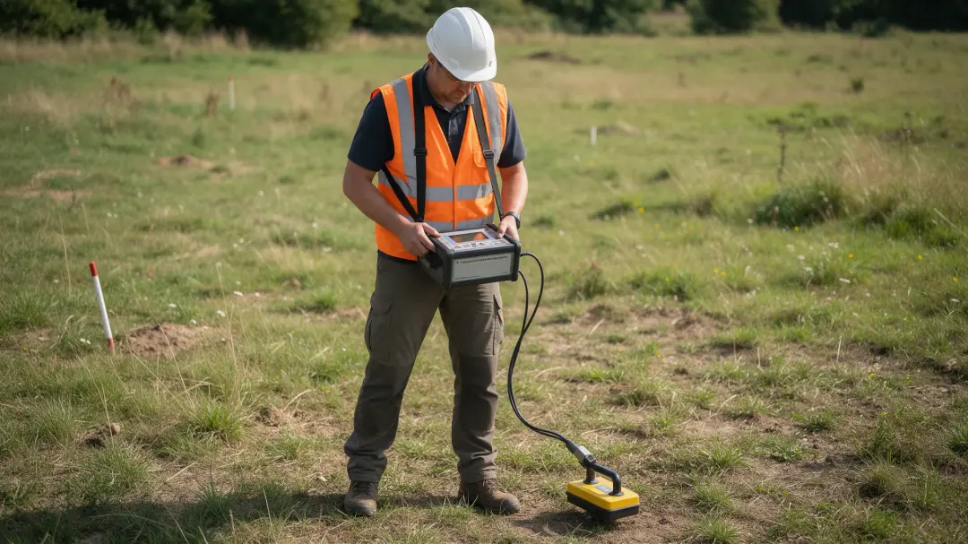
Magnetic susceptibility describes how strongly a material becomes magnetised in an applied field. Understanding the physics behind magnetic susceptibility explains why iron minerals, grain size and temperature affect measurements, and why a soil reading is more than a simple measure of its iron content.
What Does Magnetic Susceptibility Mean?
In the simplest linear model, magnetisation M equals susceptibility κ multiplied by field strength H: M = κH. Magnetisation expresses the magnetic moment per unit volume; susceptibility expresses the material’s response. A larger positive susceptibility means a stronger induced magnetisation under the same weak field.
This relationship is useful within its assumptions. Some minerals respond differently as the field changes, and a specimen can retain magnetisation after a field is removed. Low-field susceptibility describes a particular response under specified measuring conditions; it does not capture every aspect of magnetic behaviour.
Electrons Provide the Microscopic Explanation
Magnetic moments arise from electron spin and orbital motion. The way electrons occupy atomic states determines whether their moments cancel, reinforce one another or respond weakly to an external field. Crystal structure influences how neighbouring moments interact.
A rock is a mixture of minerals rather than a single ideal material. Its measured susceptibility combines their contributions, weighted by their amounts and affected by their arrangement. Two specimens with similar chemical iron concentrations can have different responses if their iron is held in different minerals. Chemistry alone cannot predict the measurement reliably.
Diamagnetism, Paramagnetism and Ferrimagnetism
Diamagnetic materials develop a weak magnetisation opposing the applied field, giving negative susceptibility. Quartz and calcite are geological examples. Paramagnetic minerals contain moments that partially align with the field but are disrupted by thermal motion; their susceptibility is generally positive and comparatively weak.

Ferrimagnetic minerals, including magnetite, contain opposing magnetic sublattices whose moments do not cancel completely. Their net response can dominate the surrounding rock. Ferromagnetism also involves strong collective alignment, but magnetite is more accurately described as ferrimagnetic. These distinctions explain why a small magnetic fraction can be influential within largely weakly magnetic sediment.
Why a Little Magnetite Can Have a Large Effect
The University of Texas expedition methods published in September 2025 reproduce reference mass-specific susceptibility ranges of 20,000–110,000 × 10⁻⁸ m³/kg for magnetite, compared with approximately −0.5 to −0.6 × 10⁻⁸ m³/kg for quartz. These are established reference values reported in a recent document, rather than new measurements of every natural rock. Source: UT-GOM2-2 expedition methods, 2025.
This contrast explains why small changes in magnetite abundance can outweigh larger changes in quartz. It does not provide a universal conversion to magnetite percentage. Grain properties, other magnetic minerals and the measuring method still matter. Mineralogical interpretations are stronger when supported by additional laboratory tests.
Grain Size and Magnetic Domains
Magnetic minerals may contain one domain or several domains with different magnetisation directions. Domain walls can move when a field is applied, contributing to the response. Larger grains, small stable grains and extremely fine particles therefore need not behave alike, even with identical mineral chemistry.
Very fine particles may be superparamagnetic: thermal fluctuations cause their moments to change direction over the measurement timescale. Their response can depend on how rapidly the instrument’s field alternates. Frequency-dependent measurements help investigate these particles, but require consideration of frequency range, temperature and mineral mixture.
Temperature Changes Magnetic Behaviour
Thermal energy competes with magnetic ordering. Magnetite’s Curie temperature is approximately 580°C, above which its ferrimagnetic ordering is lost. Temperature-dependent susceptibility can help identify magnetic phases, although laboratory heating may also oxidise or otherwise alter a specimen. Source: IODP rock-magnetic data report.

That temperature is a material property, not the temperature a field survey uses. Enhanced soil susceptibility does not prove the soil reached 580°C. Burning-related changes depend on oxygen supply, duration, starting minerals and cooling conditions. Mineral transformation and acquisition of remanent magnetisation are separate processes that should not be conflated.
Volume and Mass Susceptibility Use Different Units
Volume susceptibility is dimensionless in SI because magnetisation and field strength both have units of amperes per metre. Mass-specific susceptibility divides volume susceptibility by density and is expressed in cubic metres per kilogram. Instruments may display scaled values, so the multiplier must accompany a reported number.
A field reading and a laboratory result should not be compared just because both are labelled susceptibility. Their units, sample preparation, density correction and sensor geometry may differ. Recording these details prevents a difference caused by reporting conventions from being mistaken for geological change.
Direction Matters in Some Materials
Susceptibility need not be identical in every direction. Elongated grains, mineral alignment and rock fabric can produce anisotropy: the response measured along one axis differs from the response along another. A laboratory investigation can rotate an oriented specimen and represent those differences with a susceptibility tensor. The result may contribute evidence about sediment alignment or deformation, although its interpretation depends on which minerals carry the signal.
A bulk field measurement should not automatically be read as a fabric analysis. Orientation, specimen shape and the strength of the applied field may influence a comparison between samples. If a geological question concerns directional structure, preserve the sample’s original orientation during collection and state it in the records. An unoriented handful of soil can still give a useful bulk measurement, but it has lost information needed to investigate the original alignment. Choosing the measurement before sampling protects that information.
How a Susceptibility Meter Uses This Physics
A measuring coil creates a weak alternating field and detects how a specimen changes its electromagnetic response. A laboratory sensor controls the sample position; a surface probe interrogates a shallow, uneven volume of ground. Calibration and zero measurements separate sample response from instrument drift and the empty-sensor signal.
The method described by Pre-Construct Geophysics uses a Bartington MS2 meter and MS2D loop probe for preliminary topsoil prospecting. This investigates near-surface magnetic variation. It measures a different quantity from gradiometry, which records differences in the surrounding magnetic field. Understanding that distinction helps match an investigation to its objective.
Summary
Magnetic susceptibility connects atomic-scale behaviour with measurable contrasts in soil and rock. Mineral type, grain structure, temperature and reporting units influence the result. For site investigation, the useful question is how those contrasts guide further survey, rather than whether one high reading proves a buried feature.
Explore how Pre-Construct Geophysics applies these principles to shallow topsoil prospecting and the identification of areas for closer investigation.
Magnetic Susceptibility